Deep Learning with Python keynotes: 机器学习/深度学习基础

Deep Learning with Python keynotes & pratice
«Deep Learning with Python» 书中基础部分读书笔记及实践
Machine learning is, technically: searching for useful representa-tions of some input data, within a predefined space of possibilities, using guidance from a feedback signal.
A machine-learning model transforms its input data into meaningful outputs, a process that is “learned” from exposure to known examples of inputs and outputs. Therefore, the central problem in machine learning and deep learning is to meaningfully transform data: in other words, to learn useful representations of the input data at hand—representations that get us closer to the expected output. Before we go any further: what’s a representation? At its core, it’s a different way to look at data—to represent or encode data.
Learning, in the context of machine learning, describes an automatic search process for better representations.
Deep learning is, technically: a multistage way to learn data representations.
The deep in deep learning isn’t a reference to any kind of deeper understanding achieved by the approach; rather, it stands for this idea of successive layers of representations. How many layers contribute to a model of the data is called the depth of the model. Other appropriate names for the field could have been layered representations learning and hierarchical representations learning.
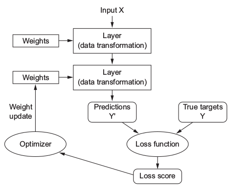
The specification of what a layer does to its input data is stored in the layer’s weights, which in essence are a bunch of numbers.
To control the output of a neural network, you need to be able to measure how far this output is from what you expected. This is the job of the loss function of the network, also called the objective function. The loss function takes the predictions of the network and the true target (what you wanted the network to output) and computes a distance score, capturing how well the network has done
The fundamental trick in deep learning is to use this score as a feedback signal to
adjust the value of the weights a little, in a direction that will lower the loss score.
This adjustment is the job of the optimizer, which implements what’s called the Backpropagation algorithm: the central algorithm in deep learning.
- Layers, which are combined into a network (or model)
- The input data and corresponding targets
- The loss function, which defines the feedback signal used for learning
- The optimizer, which determines how learning proceeds
Initially, the weights of the network are assigned random values, so the network merely implements a series of random transformations. Naturally, its output is far from what it should ideally be, and the loss score is accordingly very high. But with every example the network processes, the weights are adjusted a little in the correct direction, and the loss score decreases. This is the training loop, which, repeated a sufficient number of times (typically tens of iterations over thousands of examples), yields weight values that minimize the loss function. A network with a minimal loss is one for which the outputs are as close as they can be to the targets: a trained network.
Overfitting: the fact that machine-learning models tend to perform worse on new data than on their training data.
Tensor: At its core, a tensor is a container for data—almost always numerical data. So, it’s a container for numbers. You may be already familiar with matrices, which are 2D tensors: tensors are a generalization of matrices to an arbitrary number of dimensions (note that in the context of tensors, a dimension is often called an axis).
Scalar: Only one number
0D tensor, 0 axis.
x = np.array(1), x.ndim = 0.
Vector: An array of numbers
1D tensor, 1 axis.
x = np.array([1, 2, 3]), x.ndim = 1.
Matrices: An array of Vectors
2D tensor: 2 axes.
x = np.array([[1, 2, 3], [4, 5, 6], [7, 8, 9], [10, 11, 12]]}, x.ndim = 2.
4D tensor: An array of Matrices or an array of 3D tensors.
5D tensor: An array of 4D tensors.
…
…
…
Tensor attributes: Number of axes (rank), Shape, Data type
0D tensor:
x = np.array(1), x.shape = ().
1D tensor:
x = np.array([1, 2, 3, 4, 5]), x.shape = (1).
2D tensor:
    x = np.array([
        [1, 3, 6, 2],
        [3, 5, 6, 8],
        [6, 7, 7, 6],
        [2, 3, 4, 7],
        [8, 4, 4, 9]]),
x.shape = (5, 4).
3D tensor:
    x = np.array([[
        [1, 3, 6, 2],
        [3, 5, 6, 8],
        [6, 7, 7, 6],
        [2, 3, 4, 7],
        [8, 4, 4, 9]],
        [[1, 3, 6, 2],
        [3, 5, 6, 8],
        [6, 7, 7, 6],
        [2, 3, 4, 7],
        [8, 4, 4, 9]],
        [[1, 3, 6, 2],
        [3, 5, 6, 8],
        [6, 7, 7, 6],
        [2, 3, 4, 7],
        [8, 4, 4, 9]]]),
    x.shape = (3, 5, 4).
Data tensor examples:
Vector data— 2D tensors of shape (samples, features)
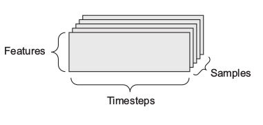
Timeseries data or sequence data— 3D tensors of shape (samples, timesteps,
features)
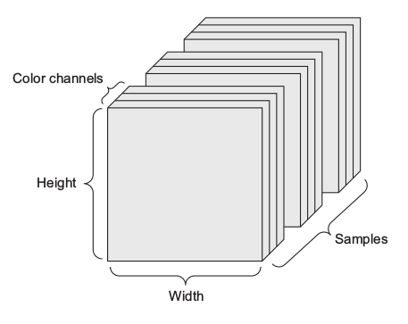
Images— 4D tensors of shape (samples, height, width, channels) or (samples,
channels, height, width)
Video— 5D tensors of shape (samples, frames, height, width, channels) or
(samples, frames, channels, height, width)
Tensor operations
Element-wise operation
Operations that are applied independently to each entry in the tensors being considered.
Broadcasting
- Axes (called broadcast axes) are added to the smaller tensor to match the ndim of the larger tensor.
- The smaller tensor is repeated alongside these new axes to match the full shape of the larger tensor.
E.g: x(32, 10), y(10) -> broadcast(x, y) => x(32, 10), y(32, 10)
Tensor dot
Also called tensor product. Dot product between two vectors is a scalar and that only
vectors with the same number of elements are compatible for a dot product. Consider the matrix multiplication.
x = [[1, 2],[3, 4]]
y = [[1, 2], [3, 4], [5, 6]]
z = x * y
x: 2 x 3, y: 3 x 3
X has 2 rows and 3 columns, and y has 3 rows and 3 columns. The number of rows of x equal the number of columns of y, so it can be multiplied.
Tensor reshaping
Reshaping a tensor means rearranging its rows and columns to match a target shape.
E.g: x = [[1, 2], [3, 4], [5, 6]], x.reshape(2, 3) => x = [[1, 2, 3], [4, 5, 6]]
Neural networks consist entirely of chains of tensor operations and that all of these tensor operations are just geometric transformations of the input data. It follows that you can interpret a neural network as a very complex geometric transformation in a high-dimensional space, implemented via a long series of simple steps.
Engine of neural networks: gradient-based optimization
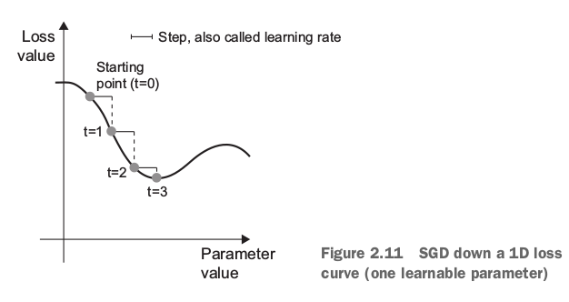
Mini-batch stochastic gradient descent
As you can see, intuitively it’s important to pick a reasonable value for the step factor.
If it’s too small, the descent down the curve will take many iterations, and it could get
stuck in a local minimum. If step is too large, your updates may end up taking you to
completely random locations on the curve.
Note that a variant of the mini-batch SGD algorithm would be to draw a single sample and target at each iteration, rather than drawing a batch of data. This would be true SGD (as opposed to mini-batch SGD ). Alternatively, going to the opposite extreme, you could run every step on all data available, which is called batch SGD . Each update would then be more accurate, but far more expensive. The efficient compromise between these two extremes is to use mini-batches of reasonable size.
Training loop
- Draw a batch of training samples x and corresponding targets y .
- Run the network on x (a step called the forward pass) to obtain predictions y_pred .
- Compute the loss of the network on the batch, a measure of the mismatch between y_pred and y.
- Update all weights of the network in a way that slightly reduces the loss on this batch.
Machine-learning problem types
Binary classification
Two-class classification, or binary classification, may be the most widely applied kind of machine-learning problem.
Learned:
-
You usually need to do quite a bit of preprocessing on your raw data in order to
be able to feed it—as tensors—into a neural network. Sequences of words can
be encoded as binary vectors, but there are other encoding options, too.
- Stacks of Dense layers with relu activations can solve a wide range of problems (including sentiment classification), and you’ll likely use them frequently.
- In a binary classification problem (two output classes), your network should end with a Dense layer with one unit and a sigmoid activation: the output of your network should be a scalar between 0 and 1, encoding a probability.
-
With such a scalar sigmoid output on a binary classification problem, the loss
function you should use is binary_crossentropy .
-
The rmsprop optimizer is generally a good enough choice, whatever your prob-
lem. That’s one less thing for you to worry about.
-
As they get better on their training data, neural networks eventually start over-
fitting and end up obtaining increasingly worse results on data they’ve never
seen before. Be sure to always monitor performance on data that is outside of
the training set.
Multiclass classification
Learned:
-
If you’re trying to classify data points among N classes, your network should end
with a Dense layer of size N .
-
In a single-label, multiclass classification problem, your network should end
with a softmax activation so that it will output a probability distribution over the
N output classes.
-
Categorical crossentropy is almost always the loss function you should use for
such problems. It minimizes the distance between the probability distributions
output by the network and the true distribution of the targets.
-
There are two ways to handle labels in multiclass classification:
– Encoding the labels via categorical encoding (also known as one-hot encod-
ing) and using categorical_crossentropy as a loss function
– Encoding the labels as integers and using the sparse_categorical_crossentropy
loss function
-
If you need to classify data into a large number of categories, you should avoid
creating information bottlenecks in your network due to intermediate layers
that are too small.
Regression
Consists of predicting a continuous value instead of a discrete label: for instance, predicting the temperature tomorrow, given meteorological data; or predicting the time that a software project will take to complete, given its specifications.
It would be problematic to feed into a neural network values that all take wildly different ranges. The network might be able to automatically adapt to such heterogeneous data, but it would definitely make learning more difficult. A widespread best practice to deal with such data is to do feature-wise normalization: for each feature in the input data (a column in the input data matrix), you subtract the mean of the feature and divide by the standard deviation, so that the feature is centered around 0 and has a unit standard deviation.
MSE: mean squared error, the square of the difference between the predictions and the targets. This is a widely used loss function for regression problems.
MAE: mean absolute error ( MAE ), the absolute value of the difference between the predictions and the targets.
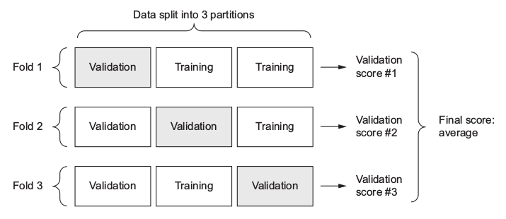
K -fold cross-validation: consists of splitting the available data into K partitions (typically K = 4 or 5), instantiating K identical models, and training each one on K – 1 partitions while evaluating on the remaining partition. The validation score for the model used is then the average of the K validation scores obtained.
E.g: 3-fold cross-validation:
There’s something wrong in the figure?
k = 4
num_validation_samples = len(data) // k
np.random.shuffle(data)
validation_scores = []
for fold in range(k):
    validation_data = data[num_validation_samples * fold :
        num_validation_samples * (fold + 1)]
    training_data = data[:num_validation_samples * fold] +
        data[num_validation_samples * (fold + 1):]
    model = get_model()
    model.train(training_data)
    validation_score = model.evaluate(validation_data)
    validation_scores.append(validation_score)

validation_score = np.average(validation_scores)

model = get_model()
model.train(data)
test_score = model.evaluate(test_data)
Learned:
- Regression is done using different loss functions than what we used for classification. Mean squared error ( MSE ) is a loss function commonly used for regression.
-
Similarly, evaluation metrics to be used for regression differ from those used for
classification; naturally, the concept of accuracy doesn’t apply for regression. A
common regression metric is mean absolute error ( MAE ).
-
When features in the input data have values in different ranges, each feature
should be scaled independently as a preprocessing step.
- When there is little data available, using K-fold validation is a great way to reliably evaluate a model.
-
When little training data is available, it’s preferable to use a small network with
few hidden layers (typically only one or two), in order to avoid severe overfitting.
Machine-learning forms
**Supervised learning **
It consists of learning to map input data to known targets (also called annotations), given a set of examples (often annotated by humans).
Unsupervised learning
Consists of finding interesting transformations of the input data without the help of any targets, for the purposes of data visualization, data compression, or data denoising, or to better understand the correlations present in the data at hand.
Self-supervised learning
Self-supervised learning is supervised learning without human-annotated labels—you can think of it as supervised learning without any humans in the loop. There are still labels involved (because the learning has to be supervised by something), but they’re generated from the input data, typically using a heuristic algorithm.
Reinforcement learning
In reinforcement learning, an agent receives information about its environment and learns to choose actions that will maximize some reward.
Data preprocessing
Data preprocessing aims at making the raw data at hand more amenable to neural
networks. This includes vectorization, normalization, handling missing values, and feature extraction.
Most common ways to prevent overfitting
- Get more training data.
- Reduce the capacity of the network.
- Add weight regularization.
- Add dropout.
import matplotlib.pyplot as plt
import numpy as np
from tensorflow import keras
from tensorflow.keras.datasets import imdb

(train_data, train_labels), (test_data,
                            test_labels) = imdb.load_data(num_words=10000)

# print(len(train_data))
# print('old_shape: {}'.format(train_data.shape))
# print(max([max(seq) for seq in train_data]))

word_index = imdb.get_word_index()
reverse_word_index = dict([(value, key)
                          for (key, value) in word_index.items()])
decoded_review = ' '.join([reverse_word_index.get(i - 3, '+')
                          for i in train_data[0]])
print(decoded_review)

def vectorize_sequences(sequences, dimension=10000):
   results = np.zeros((len(sequences), dimension))
   for i, sequence in enumerate(sequences):
       results[i, sequence] = 1
   return results

x_train = vectorize_sequences(train_data)
x_test = vectorize_sequences(test_data)

y_train = np.asarray(train_labels).astype('float32')
y_test = np.asarray(test_labels).astype('float32')

x_val = x_train[:10000]
partial_x_train = x_train[10000:]

y_val = y_train[:10000]
partial_y_train = y_train[10000:]

model = keras.models.Sequential()
model.add(keras.layers.Dense(16, activation='relu', input_shape=(10000,)))
model.add(keras.layers.Dense(16, activation='relu'))
model.add(keras.layers.Dense(1, activation='sigmoid'))
model.compile(optimizer='rmsprop', loss='binary_crossentropy', metrics=['acc'])
history = model.fit(
    partial_x_train,
    partial_y_train,
    epochs=20,
    batch_size=512,
    validation_data=(x_val, y_val)
)
history_dict = history.history
print(history_dict.keys())

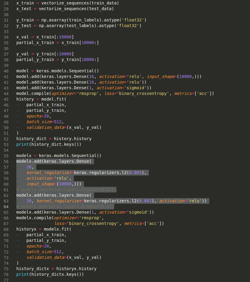
modelx = keras.models.Sequential()
modelx.add(keras.layers.Dense(
    16,
    kernel_regularizer=keras.regularizers.l2(0.001),
    activation='relu',
    input_shape=(10000,)))
# modelx.add(keras.layers.Dropout(0.5))
modelx.add(keras.layers.Dense(
    16, kernel_regularizer=keras.regularizers.l2(0.001), activation='relu'))
# modelx.add(keras.layers.Dropout(0.5))
modelx.add(keras.layers.Dense(1, activation='sigmoid'))
modelx.compile(optimizer='rmsprop',
              loss='binary_crossentropy', metrics=['acc'])
historyx = modelx.fit(
    partial_x_train,
    partial_y_train,
    epochs=20,
    batch_size=512,
    validation_data=(x_val, y_val)
)
history_dictx = historyx.history
print(history_dictx.keys())

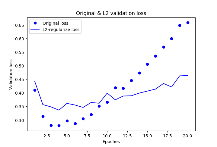
val_loss = history_dict['val_loss']
l2_val_loss = history_dictx['val_loss']
epochs = range(1, len(history_dict['acc']) + 1)
plt.plot(epochs, val_loss, 'bo', label='Original loss')
plt.plot(epochs, l2_val_loss, 'b', label='L2-regularize loss')
plt.title('Original & L2 validation loss')
plt.xlabel('Epoches')
plt.ylabel('Validation loss')
plt.legend()
plt.show()
Developing a model that does better than a baseline
Two hypotheses
- You hypothesize that your outputs can be predicted given your inputs.
- You hypothesize that the available data is sufficiently informative to learn the relationship between inputs and outputs.
Choosing the right last-layer activation and loss function for your model
| Problem type | Last-layer activation | Loss function |
| Binary classification | sigmoid | binary_crossentropy |
| Multiclass, single-label classification | softmax | categorical_crossentropy |
| Multiclass, multilabel classification | sigmoid | binary_crossentropy |
| Regression to arbitrary values | None | mse |
| Regression to values between 0 and 1 | sigmoid | mse or binary_crossentropy |
